

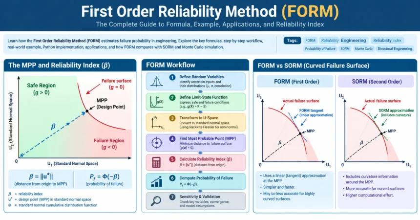
First Order Reliability Method
The First Order Reliability Method (FORM) is a probabilistic engineering method used to estimate the probability that a system, structure, component, or design will fail when its input variables are uncertain.
Instead of treating material strength, loads, dimensions, soil properties, or environmental conditions as fixed values, FORM models them as random variables and determines how close the system is to its failure condition.
The central idea is simple:
A system becomes unreliable when uncertainty allows the limit-state function to cross from the safe region into the failure region.
FORM converts this uncertainty into two important quantities:
- Reliability index (β)
- Probability of failure (Pf)
For a simple linear limit-state problem with normally distributed variables:
β=μgσg\beta = \frac{\mu_g}{\sigma_g}
and
Pf=Φ(−β)P_f = \Phi(-\beta)
where Φ\Phi is the standard normal cumulative distribution function.
FORM is particularly useful in structural reliability, geotechnical engineering, mechanical systems, offshore engineering, aerospace applications, risk analysis, and reliability-based design optimization.
What Is the First Order Reliability Method?
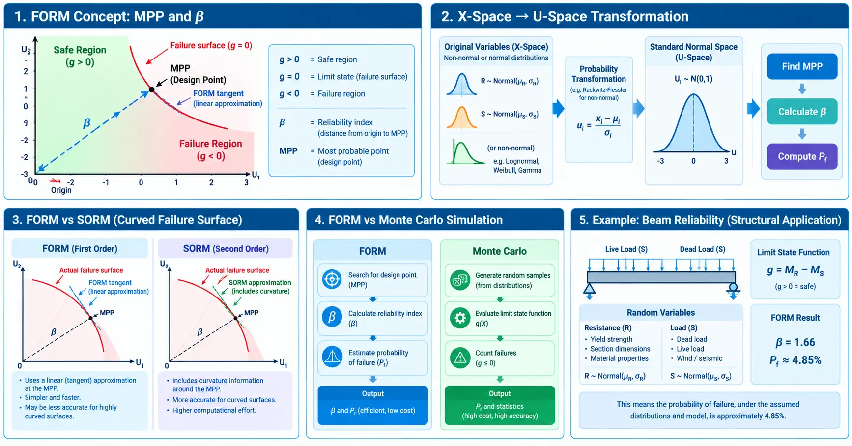
The First Order Reliability Method, commonly abbreviated as FORM, estimates failure probability by approximating the limit-state surface near its most probable point of failure.
A typical engineering reliability problem begins with a limit-state function:
g(X)g(\mathbf X)
where X\mathbf X represents uncertain input variables.
For a simple strength-versus-load problem:
g(R,S)=R−Sg(R,S)=R-S
where:
- RR = resistance or strength
- SS = applied load or demand
- g>0g>0 = safe state
- g=0g=0 = limit state
- g<0g<0 = failure state
This formulation is the foundation of FORM. Your original article uses the same resistance-minus-load framework.
A simple way to visualize FORM
             SAFE REGION
                g > 0

                  ●
                 /
                /
---------------/------------- Failure surface
              /
             /
            ●  Most Probable
               Point (MPP)

        ○ Origin in U-space
The objective is not simply to find any point where failure occurs.
FORM searches for the failure point closest to the origin in standardized probability space.
That point is called the:
Most Probable Point (MPP)
or
Design Point.
The distance from the origin to this point is the reliability index β.
Why Is FORM Important?
Traditional engineering calculations often use deterministic quantities such as a factor of safety.
For example:
FS=RSFS=\frac{R}{S}
A factor of safety can tell you how much greater the nominal resistance is than the nominal demand.
However, it does not directly describe how uncertainty in RR and SS changes the probability of failure.
Consider two designs:
| Design | Mean Resistance | Mean Load | Variability |
|---|---|---|---|
| A | High | Moderate | Low |
| B | High | Moderate | High |
A deterministic calculation might suggest that both designs have similar safety margins.
A reliability analysis can show that Design B has a substantially different failure probability because its uncertainty is larger.
This is one of the major reasons reliability methods are useful.
FORM Terminology You Need to Know
Before calculating FORM, several concepts need to be clear.
| Term | Meaning |
|---|---|
| Random variable | An uncertain engineering quantity |
| Limit-state function | Mathematical definition of safe/failure conditions |
| Failure domain | Region where g(X)<0g(X)<0 |
| Safe domain | Region where g(X)>0g(X)>0 |
| Design point | Most probable failure point |
| MPP | Most Probable Point |
| Reliability index | Distance from origin to MPP |
| Probability of failure | Probability that g(X)≤0g(X)\leq0 |
| U-space | Standardized normal probability space |
| X-space | Original physical variable space |
| Direction cosines | Sensitivity direction of the design point |
First Order Reliability Method Formula
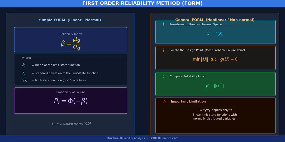
The formula depends on whether the reliability problem is simple and linear or requires a full FORM algorithm.
Simple FORM reliability index formula
For a linear limit-state function with normally distributed variables:
β=μgσg\boxed{\beta=\frac{\mu_g}{\sigma_g}}
where:
- μg\mu_g = mean of the limit-state function
- σg\sigma_g = standard deviation of the limit-state function
The probability of failure is:
Pf=Φ(−β)\boxed{P_f=\Phi(-\beta)}
Your original article identifies these as the primary formulas for the simple normal-variable case.
Important limitation
The equation
β=μgσg\beta=\frac{\mu_g}{\sigma_g}
should not be treated as the universal FORM formula.
It works directly for appropriate linear-normal cases.
For nonlinear limit-state functions, FORM generally requires transformation into standard normal space and an iterative search for the design point.
Standard Deviation of a Limit-State Function
Suppose:
g=R−Sg=R-S
and RR and SS are independent.
Then:
μg=μR−μS\mu_g=\mu_R-\mu_S
and
σg=σR2+σS2\sigma_g=\sqrt{\sigma_R^2+\sigma_S^2}
Therefore:
β=μR−μSσR2+σS2\boxed{ \beta= \frac{\mu_R-\mu_S} {\sqrt{\sigma_R^2+\sigma_S^2}} }
This is one of the easiest FORM cases to solve analytically.
What if the variables are correlated?
If RR and SS are correlated:
Var(R−S)=σR2+σS2−2ρRSσRσSVar(R-S)= \sigma_R^2+\sigma_S^2-2\rho_{RS}\sigma_R\sigma_S
Therefore:
β=μR−μSσR2+σS2−2ρRSσRσS\boxed{ \beta= \frac{\mu_R-\mu_S} {\sqrt{ \sigma_R^2+\sigma_S^2 -2\rho_{RS}\sigma_R\sigma_S }} }
Ignoring correlation can produce a misleading reliability estimate when the variables are statistically dependent.
FORM Workflow
A practical FORM calculation can be represented as:
        Define engineering problem
                  │
                  ▼
        Identify random variables
                  │
                  ▼
        Define limit-state function
                  │
                  ▼
       Specify distributions
                  │
                  ▼
       Transform X-space → U-space
                  │
                  ▼
        Search for design point
                  │
                  ▼
        Find Most Probable Point
                  │
                  ▼
       Calculate reliability index β
                  │
                  ▼
         Calculate probability Pf
                  │
                  ▼
        Perform sensitivity analysis
                  │
                  ▼
        Validate if necessary
The original article describes essentially this sequence, including defining random variables, transforming them to standard normal space, locating the MPP, linearizing the limit-state function, and calculating β.
Step 1: Define the Random Variables
Engineering quantities are rarely perfectly deterministic.
Examples include:
Structural engineering
- Yield strength
- Concrete compressive strength
- Member dimensions
- Dead load
- Live load
- Wind load
- Fatigue parameters
Geotechnical engineering
- Cohesion cc
- Friction angle ϕ\phi
- Unit weight γ\gamma
- Groundwater level
- Surcharge
Mechanical engineering
- Material strength
- Operating temperature
- Pressure
- Fatigue life
- Manufacturing tolerance
The original article identifies these types of uncertainty as important inputs to FORM.
Step 2: Define the Limit-State Function
The limit-state function separates safe and failure conditions.
For a structural member:
g(X)=R(X)−S(X)g(X)=R(X)-S(X)
The interpretation is:
g(X) > 0   →   Safe

g(X) = 0   →   Limit state

g(X) < 0   →   Failure
The exact definition depends on the engineering problem.
For example, a beam bending limit state could be:
g(MR,MS)=MR−MSg(M_R,M_S)=M_R-M_S
where:
- MRM_R = flexural resistance
- MSM_S = bending demand
For buckling:
g=Pcr−Pg=P_{cr}-P
For bearing capacity:
g=qult−qg=q_{ult}-q
For slope stability, the function may involve several correlated soil parameters.
Step 3: Transform Variables into Standard Normal Space
FORM commonly operates in standard normal space, known as U-space.
For a normally distributed variable:
ui=xi−μiσiu_i=\frac{x_i-\mu_i}{\sigma_i}
After transformation:
Ui∼N(0,1)U_i\sim N(0,1)
The original article describes this transformation and notes that U-space has mean 0 and standard deviation 1.
For non-normal variables, a more general transformation is required.
This is where methods such as the Rackwitz-Fiessler approach become relevant.
Step 4: Find the Most Probable Point
The Most Probable Point is the point on the failure surface with the smallest distance from the origin in U-space.
Mathematically:
β=minu∥u∥\beta= \min_{\mathbf u} \left\| \mathbf u \right\|
subject to:
g(u)=0g(\mathbf u)=0
This gives FORM its geometric interpretation.
                 Failure surface
                       /
                      /
                     ● MPP
                    /
                   /
                  /
                 ○
              Origin

       Distance = β
The MPP represents the combination of uncertain variables that is most likely to produce failure under the FORM approximation.
Step 5: Linearize the Limit-State Function
Suppose the actual failure surface is curved:
Actual failure surface

          )
        )
      )
    )
  )
FORM approximates it locally around the MPP:
FORM approximation

       /
      /
     /
    /
   /
This is the “first-order” part of the method.
The local approximation can be written as:
g(u)≈∇g(u∗)T(u−u∗)g(\mathbf u) \approx \nabla g(\mathbf u^*)^T (\mathbf u-\mathbf u^*)
where u∗\mathbf u^* represents the design point.
Step 6: Calculate the Reliability Index
Once the design point is known:
β=u1∗2+u2∗2+⋯+un∗2\boxed{ \beta= \sqrt{ u_1^{*2}+u_2^{*2}+\cdots+u_n^{*2} } }
The original article describes β as the distance from the origin to the design point.
A larger β generally corresponds to a smaller probability of failure under the FORM assumptions.
Step 7: Calculate Probability of Failure
The FORM approximation is:
Pf=Φ(−β)\boxed{P_f=\Phi(-\beta)}
For example:
| β | Approximate PfP_f |
|---|---|
| 1.0 | 15.87% |
| 1.5 | 6.68% |
| 2.0 | 2.28% |
| 2.5 | 0.62% |
| 3.0 | 0.135% |
| 3.5 | 0.023% |
| 4.0 | 0.0032% |
These values illustrate the nonlinear relationship between β and failure probability.
Important: A reliability index is not itself a percentage. β and PfP_f are different quantities.
First Order Reliability Method Worked Example
Consider a structural component with uncertain resistance and load.
Assume:
R∼N(100,10)R\sim N(100,10)
and:
S∼N(70,15)S\sim N(70,15)
where the second values represent standard deviations.
The limit-state function is:
g=R−Sg=R-S
These are the same base assumptions used in the original article’s solved example.
Step 1: Calculate mean limit state
μg=μR−μS\mu_g=\mu_R-\mu_S μg=100−70=30\mu_g=100-70=30
Step 2: Calculate standard deviation
Assuming independence:
σg=σR2+σS2\sigma_g= \sqrt{\sigma_R^2+\sigma_S^2} =102+152=\sqrt{10^2+15^2} =325=\sqrt{325} σg≈18.03\sigma_g\approx18.03
The original article gives the same intermediate result.
Step 3: Calculate β
β=3018.03\beta= \frac{30}{18.03} β≈1.66\boxed{\beta\approx1.66}
Step 4: Calculate probability of failure
Pf=Φ(−1.66)P_f=\Phi(-1.66) Pf≈0.0485\boxed{P_f\approx0.0485}
Therefore:
Pf≈4.85%\boxed{P_f\approx4.85\%}
The original calculation reports β ≈ 1.66 and PfP_f ≈ 4.85%.
What Does the Example Actually Mean?
The result should not be interpreted as “the structure will definitely fail 4.85% of the time.”
Rather, under the assumed probability distributions, independence assumption, limit-state model, and FORM/normal approximation, the estimated probability of the event R−S≤0R-S\leq0 is approximately 4.85%.
That distinction matters.
A reliability result is only as credible as the:
- Input distributions
- Statistical dependence assumptions
- Limit-state model
- Parameter estimates
- Numerical solution
- Model uncertainty treatment
Python Implementation of a Simple FORM Calculation
A basic normal-variable example can be implemented with Python.
import math
from statistics import NormalDist

# Mean values
mu_R = 100
mu_S = 70

# Standard deviations
sigma_R = 10
sigma_S = 15

# Mean and standard deviation of g = R - S
mu_g = mu_R - mu_S
sigma_g = math.sqrt(sigma_R**2 + sigma_S**2)

# Reliability index
beta = mu_g / sigma_g

# Probability of failure
pf = NormalDist().cdf(-beta)

print(f"Mean limit state: {mu_g:.2f}")
print(f"Std. deviation: {sigma_g:.2f}")
print(f"Reliability index: {beta:.3f}")
print(f"Probability of failure: {pf:.4%}")
Expected output:
Mean limit state: 30.00
Std. deviation: 18.03
Reliability index: 1.664
Probability of failure: 4.81%
Small numerical differences can occur because of rounding.
Why this code is useful
It demonstrates the simplest analytical FORM case.
It is not a complete general-purpose FORM solver.
For nonlinear engineering models, you need:
- Distribution transformations
- Gradient evaluation
- Correlation handling
- Design-point optimization
- Convergence criteria
- Numerical stability checks
A More Realistic First Order Reliability Method (FORM) Architecture
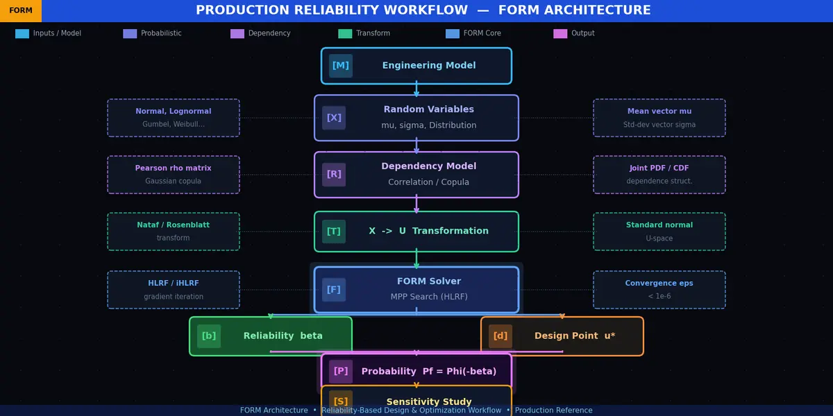
A production reliability workflow can be organized like this:
              ┌──────────────────┐
              │ Engineering Model│
              └────────┬─────────┘
                       │
                       ▼
             ┌────────────────────┐
             │ Random Variables   │
             │ μ, σ, Distribution │
             └─────────┬──────────┘
                       │
                       ▼
             ┌────────────────────┐
             │ Dependency Model   │
             │ Correlation / Copula│
             └─────────┬──────────┘
                       │
                       ▼
             ┌────────────────────┐
             │ X → U Transformation│
             └─────────┬──────────┘
                       │
                       ▼
             ┌────────────────────┐
             │ FORM Solver        │
             │ MPP Search         │
             └─────────┬──────────┘
                       │
             ┌─────────┴─────────┐
             ▼                   ▼
       Reliability β        Design Point
             │                   │
             └─────────┬─────────┘
                       ▼
                 Probability Pf
                       │
                       ▼
              Sensitivity Study
                       │
                       ▼
                Engineering Decision
This architecture is useful when FORM becomes part of a larger reliability-based design or optimization workflow.
Hasofer-Lind Reliability Index
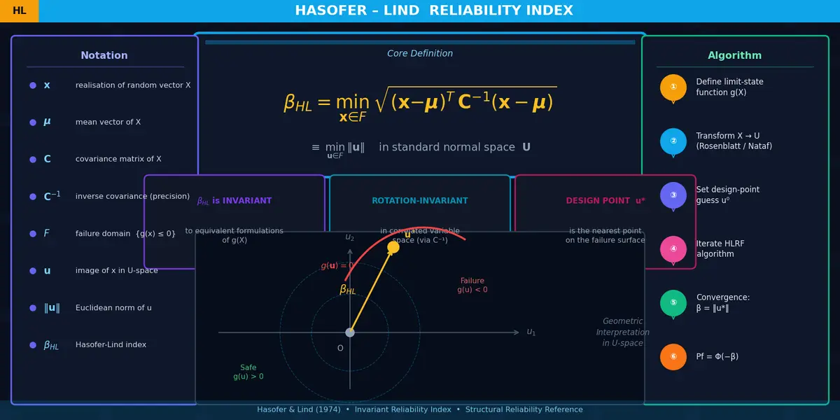
The Hasofer-Lind reliability index provides the geometric foundation of FORM.
For a problem represented in standard normal space:
β=minu:g(u)=0uTu\boxed{ \beta=\min_{\mathbf u:g(\mathbf u)=0} \sqrt{\mathbf u^T\mathbf u} }
In other words, β is the shortest distance between the origin and the failure surface.
This is important because the reliability index should describe the geometry of the probabilistic problem rather than depend simply on how someone algebraically writes the limit-state equation.
The original article also identifies the Hasofer-Lind formulation as a central part of FORM.
Direction Cosines and Sensitivity
At the design point, the normalized gradient provides the direction cosines:
αi=∂g∂ui∥∇g∥\alpha_i= \frac{ \frac{\partial g}{\partial u_i} }{ \left\|\nabla g\right\| }
These values are useful because they indicate which standardized variables have the strongest influence on the reliability calculation near the MPP.
For example:
| Variable | α | Interpretation |
|---|---|---|
| Material strength | -0.72 | Strong influence |
| Dead load | 0.25 | Moderate influence |
| Live load | 0.61 | Strong influence |
| Dimension | 0.14 | Smaller local influence |
The signs depend on how the limit-state function is formulated.
Therefore, direction cosines should be interpreted together with the definition of gg.
Rackwitz-Fiessler Algorithm
Real engineering variables are often not normally distributed.
Common distributions include:
- Lognormal
- Weibull
- Gumbel
- Gamma
- Beta
The original article specifically identifies these distributions and discusses the Rackwitz-Fiessler method for handling non-normal variables.
The Rackwitz-Fiessler approach transforms a non-normal variable into an equivalent normal representation at the current iteration point.
Conceptually:
Original variable
       │
       ▼
Non-normal distribution
       │
       ▼
Equivalent normal representation
       │
       ▼
U-space
       │
       ▼
FORM iteration
       │
       └──────► Update transformation
This transformation is one reason practical FORM implementations are more complicated than simply calculating:
β=μgσg\beta=\frac{\mu_g}{\sigma_g}
FORM for Nonlinear Limit-State Functions
Consider:
g(X1,X2)=X12+X2−10g(X_1,X_2)=X_1^2+X_2-10
The failure surface is curved.
A simple mean-to-standard-deviation calculation cannot fully represent the geometry.
FORM instead:
- Defines the nonlinear limit state.
- Transforms variables into U-space.
- Searches for the MPP.
- Evaluates the gradient.
- Linearizes the surface at the MPP.
- Calculates β.
- Converts β into an approximate PfP_f.
This is where an actual FORM solver becomes necessary.
FORM vs Monte Carlo Simulation
FORM and Monte Carlo simulation solve reliability problems differently.
| Feature | FORM | Monte Carlo |
|---|---|---|
| Basic approach | Local approximation | Random sampling |
| Main output | β and PfP_f | PfP_f and statistics |
| Computational cost | Usually low | Can be very high |
| Nonlinear models | Moderate capability | Strong capability |
| Rare events | Efficient | Potentially expensive |
| Multiple failure regions | Can be difficult | Naturally handled with enough samples |
| Optimization | Useful | Often expensive |
| Implementation | Mathematically involved | Conceptually simple |
| Local geometry | Important | Less dependent on local geometry |
The original article identifies FORM as faster and simulation as computationally expensive for rare events, while also noting that Monte Carlo handles nonlinear behavior well.
The practical question is not “Which method is always better?”
A better question is:
Does the limit-state geometry and required accuracy make FORM an appropriate approximation?
FORM vs SORM
The Second Order Reliability Method (SORM) extends the local approximation by incorporating curvature.
FORM
Actual surface
       )
      )
     )
----/----------------
   /
  /  FORM tangent
 /
SORM
SORM attempts to account for the curvature around the design point.
| Characteristic | FORM | SORM |
|---|---|---|
| Approximation | First order | Second order |
| Surface representation | Local tangent | Local curvature |
| Computational effort | Lower | Higher |
| Curved failure surface | May lose accuracy | Better suited |
| Typical use | Initial reliability assessment | More detailed approximation |
The original article describes this distinction directly.
FORM vs Monte Carlo vs SORM: Decision Table
| Situation | Potential approach |
|---|---|
| Simple linear-normal problem | Analytical reliability calculation |
| Nonlinear but smooth limit state | FORM |
| Strong local curvature | Consider SORM |
| Extremely complex simulation model | Monte Carlo or advanced simulation |
| Multiple failure regions | Monte Carlo or specialized reliability methods |
| Very rare failure probability | FORM/SORM or rare-event simulation |
| Need detailed empirical distribution | Monte Carlo |
| Design optimization with many evaluations | FORM can be computationally attractive |
| Strong model discontinuity | Validate FORM carefully |
| Unknown or poorly characterized distributions | Improve statistical model before relying on β |
This is a method-selection framework, not a universal rule. The appropriate method depends on the model, distributions, computational budget, and required reliability accuracy.
FORM Applications in Structural Engineering
FORM can be applied to many structural limit states.
The original article lists applications including beam bending, shear, column buckling, bridge girders, reinforced concrete, steel members, wind, seismic loading, and fatigue.
Example: Beam reliability
Suppose:
g=MR−MSg=M_R-M_S
where:
- MRM_R = random bending resistance
- MSM_S = random bending demand
Possible random variables include:
Material strength
       │
       ├──► Resistance
       │
Section dimensions
       │
       └──► Resistance

Dead load ──────┐
                ├──► Bending demand
Live load ──────┘
FORM can then estimate the probability that:
MS>MRM_S>M_R
FORM in Geotechnical Engineering
Geotechnical reliability is particularly interesting because soil properties can vary substantially spatially and statistically.
The original article identifies applications such as slope stability, bearing capacity, pile capacity, retaining walls, embankments, settlement, and seepage.
Typical random variables include:
c,ϕ,γ,q,Hwc,\phi,\gamma,q,H_w
where:
- cc = cohesion
- ϕ\phi = friction angle
- γ\gamma = unit weight
- qq = surcharge
- HwH_w = groundwater-related parameter
For a slope:
g(c,ϕ,γ,H,…)=FS−1g(c,\phi,\gamma,H,\ldots) = FS-1
can be used as a conceptual limit-state formulation.
Here:
g>0g>0
corresponds to:
FS>1FS>1
while:
g<0g<0
corresponds to:
FS<1FS<1
The exact formulation depends on the slope-stability model and how uncertainty is represented.
Real-World Use Cases for FORM
FORM is useful whenever an engineering decision depends on uncertain inputs.
Use case 1: Bridge reliability
Uncertain:
- Vehicle loading
- Material strength
- Fatigue parameters
- Member dimensions
- Environmental exposure
Possible limit states:
- Flexural failure
- Shear failure
- Fatigue
- Buckling
Use case 2: Offshore structure
Uncertain:
- Wave height
- Wind speed
- Structural resistance
- Material properties
Possible limit state:
g=R−Sg=R-S
Use case 3: Foundation
Uncertain:
- Soil cohesion
- Friction angle
- Unit weight
- Groundwater
- Foundation dimensions
Possible failure modes:
- Bearing capacity
- Sliding
- Overturning
- Settlement
Use case 4: Mechanical component
Uncertain:
- Applied stress
- Material strength
- Temperature
- Manufacturing tolerance
Possible limit state:
g=σallow−σactualg=\sigma_{allow}-\sigma_{actual}
Edge Cases Where FORM Needs Extra Care
FORM is powerful, but its assumptions matter.
1. Highly nonlinear failure surface
If the failure surface has strong curvature near the MPP, the first-order approximation may not adequately represent the failure domain.
Consider SORM or simulation-based validation.
2. Multiple design points
A system may have multiple regions where failure is likely.
A single MPP may not adequately represent the entire failure probability.
             Failure region

          ● MPP 1

       ○ Origin

                    ● MPP 2
In such cases, multi-modal reliability analysis or simulation may be required.
3. Discontinuous models
If:
g(X)g(X)
contains abrupt discontinuities, numerical gradients may become unreliable.
FORM relies heavily on local information around the design point.
4. Strongly dependent variables
Assuming independence when variables are actually correlated can distort the reliability calculation.
Correlation should be explicitly modeled where justified by data or engineering knowledge.
5. Poorly characterized distributions
A highly precise β calculated from poor statistical assumptions can create false confidence.
Better input data can sometimes improve the reliability assessment more than choosing a more sophisticated numerical algorithm.
Common FORM Mistakes
Mistake 1: Treating β as probability
Incorrect:
β = 3 means 3% failure probability.
Correct:
Pf=Φ(−3)P_f=\Phi(-3)
which is approximately 0.135%.
Mistake 2: Assuming β = μg/σg always
This shortcut applies to appropriate linear-normal formulations.
General nonlinear FORM requires a design-point search.
Mistake 3: Ignoring correlation
For dependent variables, covariance terms matter.
Mistake 4: Ignoring model uncertainty
Material and load uncertainty are not necessarily the only sources of uncertainty.
Model error may also be important.
Mistake 5: Reporting β without assumptions
A reliability result should ideally state:
- Random variables
- Distributions
- Means
- Standard deviations
- Correlations
- Limit-state function
- Transformation method
- FORM algorithm
- Convergence criteria
- β
- PfP_f
What Should a FORM Result Report Look Like?
A technically useful reliability report could use this format:
| Parameter | Result |
|---|---|
| Limit state | g(X)=R−Sg(X)=R-S |
| Random variables | R, S |
| Distribution | Normal |
| μR | 100 |
| σR | 10 |
| μS | 70 |
| σS | 15 |
| Correlation | 0 |
| Reliability index | 1.66 |
| Probability of failure | ≈4.85% |
| Method | FORM |
| Approximation | First order |
This is much more informative than reporting β alone.
Advantages of the First Order Reliability Method
FORM remains useful because it combines mathematical insight with relatively low computational cost.
Important advantages include:
- Provides a reliability index
- Estimates probability of failure
- Usually requires far fewer model evaluations than brute-force simulation
- Supports sensitivity analysis
- Works naturally with reliability-based design
- Can handle multiple random variables
- Can incorporate non-normal distributions through transformations
- Provides a useful geometric interpretation
- Can be integrated with optimization workflows
The original article also highlights speed, sensitivity analysis, code calibration, and reliability-based optimization as important advantages.
Limitations of FORM
FORM should not be treated as an exact probability calculator for every engineering problem.
Important limitations include:
- First-order approximation
- Sensitivity to distribution assumptions
- Potential difficulty with multiple design points
- Potential problems with strongly nonlinear limit states
- Dependence on numerical convergence
- Sensitivity to gradient calculations
- Possible errors when the failure surface is highly curved
These limitations are also identified in the original article.
When Should You Use FORM?
Use FORM when:
- The engineering model is reasonably smooth.
- The failure surface can be approximated locally.
- Input distributions can be characterized reasonably well.
- You need an efficient reliability estimate.
- You need a design point for sensitivity analysis.
- You are performing reliability-based design optimization.
Consider additional methods when:
- Failure regions are highly disconnected.
- The model is discontinuous.
- Strong nonlinearities dominate.
- Multiple MPPs exist.
- You require validation of a very low failure probability.
FORM Implementation Checklist
Before trusting a FORM result, check the following:
Model
- Is the limit-state function physically correct?
- Are all relevant failure modes included?
- Is model uncertainty considered?
Probability model
- Are distributions justified?
- Are means and standard deviations based on appropriate data?
- Are correlations known?
- Are non-normal distributions transformed correctly?
Numerical method
- Did the solver converge?
- Is the design point physically meaningful?
- Is the gradient reliable?
- Were alternative starting points tested where appropriate?
Validation
- Is FORM appropriate for the failure surface?
- Should SORM be considered?
- Should Monte Carlo simulation be used as a validation check?
Frequently Asked Questions
What is the First Order Reliability Method?
The First Order Reliability Method (FORM) is a probabilistic reliability-analysis technique that estimates failure probability by approximating a limit-state function around its most probable point of failure.
What is the FORM formula?
For a suitable linear-normal problem:
β=μgσg\beta=\frac{\mu_g}{\sigma_g}
and:
Pf=Φ(−β)P_f=\Phi(-\beta)
For nonlinear problems, FORM generally requires an iterative design-point calculation.
What is the reliability index in FORM?
The reliability index β represents the shortest distance between the origin and the failure surface in standard normal space.
What does a higher β mean?
Under the usual FORM interpretation, a larger β corresponds to a smaller estimated probability of failure.
What is the MPP in FORM?
The Most Probable Point is the point on the failure surface closest to the origin in standard normal space.
What is the difference between FORM and SORM?
FORM uses a first-order local approximation, while SORM incorporates second-order curvature information around the design point.
What is the difference between FORM and Monte Carlo?
FORM searches for a critical design point and approximates the failure surface locally. Monte Carlo estimates failure probability by sampling the underlying random variables.
Can FORM handle non-normal variables?
Yes. Practical FORM implementations can transform non-normal variables into an appropriate normal-space representation. The Rackwitz-Fiessler approach is one such method.
Where is FORM used?
Common applications include:
- Structural reliability
- Geotechnical engineering
- Bridge reliability
- Foundation analysis
- Offshore structures
- Aerospace reliability
- Mechanical reliability
- Risk-based design
These application areas are also covered in the original article.
Key Takeaways
The First Order Reliability Method provides a practical way to quantify engineering uncertainty.
The central workflow is:
Random Variables→Limit State→U-Space→MPP→β→Pf\boxed{ \text{Random Variables} \rightarrow \text{Limit State} \rightarrow \text{U-Space} \rightarrow \text{MPP} \rightarrow \beta \rightarrow P_f }
For a simple linear-normal resistance-load problem:
β=μR−μSσR2+σS2\boxed{ \beta= \frac{\mu_R-\mu_S} {\sqrt{\sigma_R^2+\sigma_S^2}} }
and:
Pf=Φ(−β)\boxed{ P_f=\Phi(-\beta) }
However, real FORM analysis is more than plugging numbers into these equations. The reliability result depends on the limit-state model, probability distributions, correlations, transformation method, design-point search, and assumptions about model uncertainty.
That is why a good FORM analysis should report not only β and PfP_f but also the assumptions and methodology used to obtain them.

AiVoogle – AI Tutorials & AI Tools
AiVoogle is an AI-focused platform sharing practical AI tutorials, AI tools, guides, reviews, and the latest trends in artificial intelligence. Our goal is to make AI simple, useful, and accessible for everyone—from beginners and creators to marketers, developers, and businesses.
The AiVoogle team researches and covers the latest AI tools and technologies to help readers discover the right tools and learn how to use AI effectively.
Focus: AI Tutorials | AI Tools | AI Guides | AI News | AI Reviews