

Sigmoid vs ReLU is more than a comparison between two mathematical functions. The activation function used inside a neural network affects gradient flow, optimization behavior, computational cost, representation learning, and ultimately how effectively a model can learn.
Sigmoid compresses every input into the range 0 to 1, making it useful when an output represents a probability. ReLU, or Rectified Linear Unit, instead returns zero for negative inputs and the input itself for positive values. Its simple gradient behavior makes it much easier to optimize in many deep networks.
The important distinction is this:
ReLU is usually a strong choice for hidden layers, while sigmoid remains highly useful for specific output-layer problems such as binary classification.
So the practical question is not simply “Which is better, sigmoid or ReLU?” It is:
“Which activation function is appropriate for this layer, architecture, optimization problem, and output representation?”
What Is an Activation Function?
A neural network layer first performs a weighted linear transformation:
z=Wx+bz = Wx + b
where:
- xx is the input vector
- WW represents learned weights
- bb is the bias
- zz is the pre-activation value
The activation function then transforms this value:
a=f(z)a = f(z)
The activation function introduces non-linearity into the network.
Without a nonlinear activation function, stacking multiple linear layers would still produce a linear transformation. In other words, adding more linear layers would not give the network the expressive power normally associated with deep learning.
Google’s Machine Learning Crash Course describes activation functions as nonlinear transformations that allow neural networks to learn complex relationships.
A simple neural-network architecture
Input
  │
  ▼
┌───────────────┐
│ Linear Layer  │
│ z = Wx + b    │
└───────┬───────┘
        │
        ▼
┌───────────────┐
│ Activation    │
│ a = f(z)      │
└───────┬───────┘
        │
        ▼
     Next Layer
The activation function is therefore part of the computational path through which information and gradients move.
What Is Sigmoid?
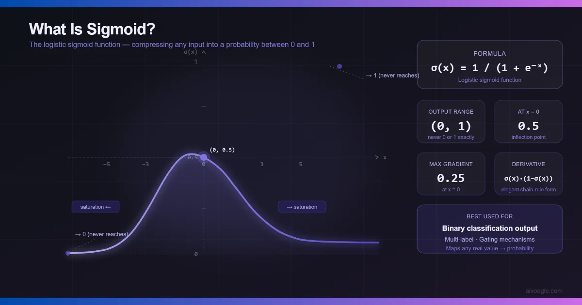
The sigmoid function, more precisely the logistic sigmoid, is defined as:
σ(x)=11+e−x\sigma(x)=\frac{1}{1+e^{-x}}
Its output always lies between 0 and 1:
0<σ(x)<10 < \sigma(x) < 1
TensorFlow defines sigmoid using the same equation and notes that large negative inputs approach 0 while large positive inputs approach 1.
Sigmoid behavior
Output
1.0 |                         ─────────
    |                    ─────
0.5 |──────────────●────
    |          ───
0.0 |────────
    +----------------------------------
          Negative   0    Positive
                    Input
At:
x=0x=0
the sigmoid output is:
σ(0)=0.5\sigma(0)=0.5
For example:
| Input | Sigmoid Output |
|---|---|
| -10 | ≈ 0.00005 |
| -5 | ≈ 0.0067 |
| -2 | ≈ 0.119 |
| 0 | 0.5 |
| 2 | ≈ 0.881 |
| 5 | ≈ 0.993 |
| 10 | ≈ 0.99995 |
This makes sigmoid particularly useful when the output needs to represent a probability-like value.
Sigmoid Derivative and the Vanishing Gradient Problem
The derivative of sigmoid has an especially convenient form:
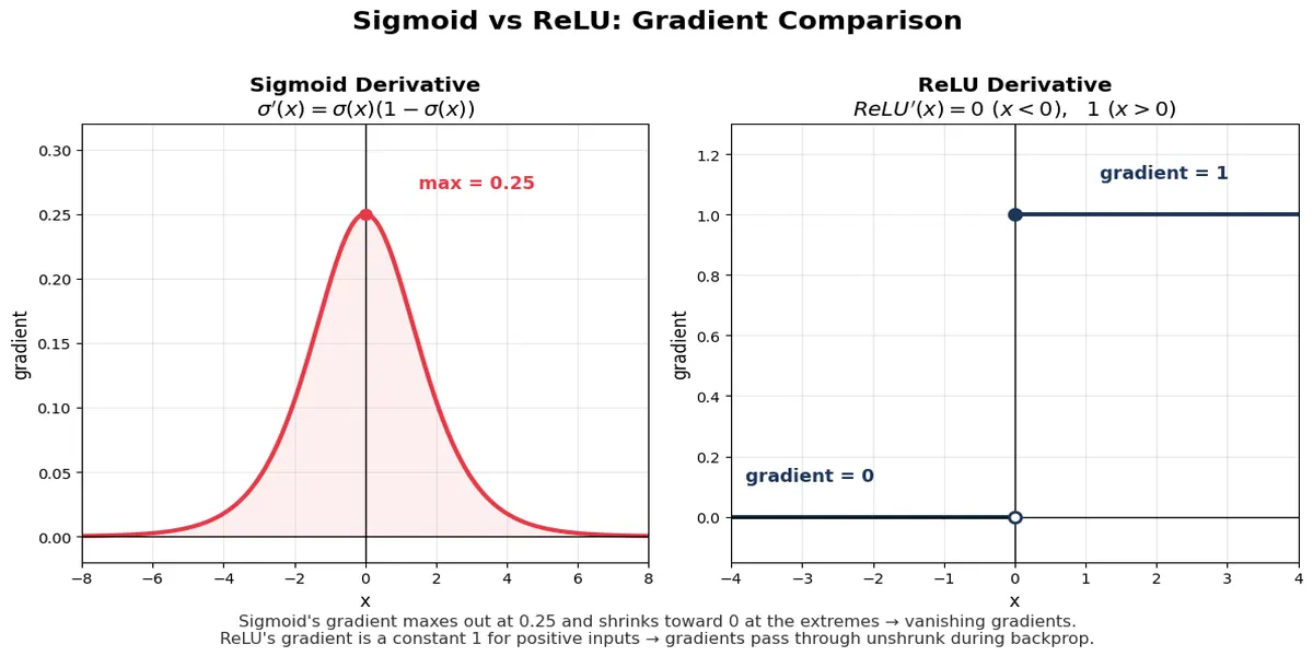
σ′(x)=σ(x)(1−σ(x))\sigma'(x)=\sigma(x)(1-\sigma(x))
The maximum derivative occurs at x=0x=0:
σ′(0)=0.25\sigma'(0)=0.25
The derivative becomes increasingly small as xx moves toward either extreme.
For example:
x = -10
sigmoid(x) ≈ 0
gradient   ≈ 0

x = 0
sigmoid(x) = 0.5
gradient   = 0.25

x = +10
sigmoid(x) ≈ 1
gradient   ≈ 0
This is called saturation.
During backpropagation, gradients are propagated through successive layers using the chain rule. If many layers contain derivatives significantly smaller than 1, multiplying those derivatives can make the gradient extremely small.
Conceptually:
∂L∂x=∂L∂a∂a∂z∂z∂x\frac{\partial L}{\partial x} = \frac{\partial L}{\partial a} \frac{\partial a}{\partial z} \frac{\partial z}{\partial x}
Across many layers, this becomes a product of many derivative terms.
If those terms are small:
0.2×0.2×0.2×0.20.2 \times 0.2 \times 0.2 \times 0.2
the resulting gradient becomes tiny.
Google identifies this as the vanishing gradient problem, where lower layers can train extremely slowly or effectively stop learning.
This is one of the primary reasons sigmoid became less attractive for deep hidden layers.
What Is ReLU?
ReLU stands for Rectified Linear Unit.
Its mathematical definition is:
ReLU(x)=max(0,x)ReLU(x)=\max(0,x)
Therefore:
ReLU(x)={0x<0xx≥0ReLU(x)= \begin{cases} 0 & x<0 \\ x & x\geq0 \end{cases}
TensorFlow uses this standard formulation for its default ReLU implementation.
ReLU behavior
Output
  ^
  |                 /
  |               /
  |             /
  |           /
0 +----------●----------------> Input
  |         /
  |
  |  0 for all negative x
Examples:
| Input | ReLU Output |
|---|---|
| -10 | 0 |
| -2 | 0 |
| -0.5 | 0 |
| 0 | 0 |
| 0.5 | 0.5 |
| 2 | 2 |
| 10 | 10 |
Unlike sigmoid, ReLU does not compress positive values into a fixed range.
Why ReLU Changed Deep Learning
ReLU’s most important advantage is not simply that it is easy to calculate.
Its key advantage comes from its gradient.
For positive inputs:
ReLU′(x)=1ReLU'(x)=1
For negative inputs:
ReLU′(x)=0ReLU'(x)=0
Ignoring the single point at zero, this means positive activations can propagate a gradient without the repeated multiplicative shrinkage associated with sigmoid’s saturated regions.
Google notes that ReLU is less susceptible to vanishing gradients than smooth functions such as sigmoid and tanh, and is also computationally simpler.
This helped make very deep neural networks substantially easier to optimize.
Sigmoid vs ReLU: The Core Mathematical Difference
The simplest way to understand the difference is to compare their derivatives.
Sigmoid
σ′(x)=σ(x)(1−σ(x))\sigma'(x)=\sigma(x)(1-\sigma(x))
Maximum derivative:
0.250.25
ReLU
ReLU′(x)={0x<01x>0ReLU'(x)= \begin{cases} 0 & x<0\\ 1 & x>0 \end{cases}
So for a positive ReLU activation, the local gradient is 1.
                 SIGMOID

gradient
  ^
.25|             ●
   |           /   \
   |         /       \
  0|────────/─────────\────────
   +--------------------------> x


                  ReLU

gradient
  ^
 1 |                  ─────────
   |
 0 |──────────────────
   +--------------------------> x
                 0
This difference has major consequences during backpropagation.
Sigmoid vs ReLU Comparison Table
| Characteristic | Sigmoid | ReLU |
|---|---|---|
| Formula | 1/(1+e−x)1/(1+e^{-x}) | max(0,x)max(0,x) |
| Output range | 0 to 1 | 0 to ∞ |
| Zero-centered | No | No |
| Positive-side gradient | ≤ 0.25 | 1 |
| Negative-side gradient | Small but non-zero | 0 |
| Saturation | Strong | Positive side does not saturate |
| Vanishing-gradient risk | High | Lower |
| Computational cost | Higher | Very low |
| Sparse activations | No | Yes |
| Typical hidden-layer use | Limited | Very common |
| Binary output | Excellent | Generally inappropriate |
| Deep hidden layers | Usually avoided | Common |
| Main failure mode | Saturation | Dead neurons |
The table illustrates an important point: neither function is universally superior.
Why ReLU Is Usually Used in Hidden Layers
Consider a simple multilayer perceptron:
Input
  │
  ▼
Dense
  │
  ▼
ReLU
  │
  ▼
Dense
  │
  ▼
ReLU
  │
  ▼
Dense
  │
  ▼
Sigmoid
  │
  ▼
Probability
For binary classification, this architecture is often conceptually appropriate:
- ReLU handles nonlinear representation learning in hidden layers.
- Sigmoid converts the final logit into a probability.
For example, suppose a fraud detection model predicts:
Fraud probability = 0.93
The final sigmoid can map a real-valued logit into a number between 0 and 1.
The hidden layers do not need their outputs restricted to 0–1. They need useful representations that can be optimized efficiently.
A Real Example: Spam Email Classification
Suppose a model receives features such as:
- number of suspicious words
- sender reputation
- number of links
- message length
- domain age
- attachment indicators
A neural network could look like:
                Email Features
                       │
                       ▼
              ┌────────────────┐
              │ Dense(128)     │
              │ ReLU           │
              └───────┬────────┘
                      │
                      ▼
              ┌────────────────┐
              │ Dense(64)      │
              │ ReLU           │
              └───────┬────────┘
                      │
                      ▼
              ┌────────────────┐
              │ Dense(1)       │
              │ Sigmoid        │
              └───────┬────────┘
                      │
                      ▼
             Spam Probability
If the final output is:
0.970.97
the model estimates a high probability for the positive class.
The important architectural decision is that sigmoid is used for the output representation, not because sigmoid is inherently superior to ReLU.
Why Sigmoid Can Be a Poor Hidden-Layer Activation
Consider a deep network with several sigmoid layers.
A neuron may produce:
z=8z=8
Then:
σ(8)≈0.9997\sigma(8)\approx0.9997
Its derivative is approximately:
0.00030.0003
That is a very small gradient.
Now imagine this effect occurring repeatedly across many layers.
The lower layers may receive only a tiny gradient signal.
This creates a difficult optimization environment:
Loss
 │
 ▼
Output Layer
 │  gradient
 ▼
Hidden Layer 4
 │  smaller gradient
 ▼
Hidden Layer 3
 │  smaller again
 ▼
Hidden Layer 2
 │  extremely small
 ▼
Hidden Layer 1
This does not mean sigmoid networks cannot be trained. They can.
It means that sigmoid’s saturation makes optimization substantially more difficult in many deep architectures.
The ReLU Problem: Dead Neurons
ReLU solves one major problem but introduces another.
For negative inputs:
ReLU(x)=0ReLU(x)=0
and:
ReLU′(x)=0ReLU'(x)=0
Suppose a neuron’s weights and bias evolve so that its pre-activation is consistently negative for the training examples.
The neuron produces:
activation = 0
gradient   = 0
It may effectively stop contributing to learning.
This phenomenon is commonly called a dead ReLU or dying ReLU.
Google’s backpropagation documentation explicitly discusses dead ReLU units and notes that lowering the learning rate can help prevent them.
Dead ReLU example
Input
  │
  ▼
Weighted Sum
  │
  │ z < 0
  ▼
ReLU
  │
  ▼
0
  │
  X
No gradient through negative branch
This is why saying “ReLU has no disadvantages” would be technically incorrect.
ReLU Variants
Researchers and framework developers have introduced several alternatives to standard ReLU.
Leaky ReLU
Leaky ReLU allows a small negative slope:
f(x)={xx>0αxx≤0f(x)= \begin{cases} x & x>0\\ \alpha x & x\leq0 \end{cases}
For example, if:
α=0.01\alpha=0.01
then:
Input   Leaky ReLU
-10     -0.10
-2      -0.02
-1      -0.01
 0       0
 2       2
The negative branch now retains a gradient.
PReLU
Parametric ReLU makes the negative slope learnable:
f(x)={xx>0αxx≤0f(x)= \begin{cases} x & x>0\\ \alpha x & x\leq0 \end{cases}
but α\alpha becomes a learned parameter.
The original PReLU research explored this approach and showed that rectifier-based architectures could be trained effectively at substantial depth.
Sigmoid vs ReLU vs Tanh
Sigmoid and ReLU are not the only activation functions worth understanding.
Tanh is defined as:
tanh(x)tanh(x)
and produces outputs between:
−1 and 1-1 \text{ and } 1
Google documents sigmoid, tanh, and ReLU as common activation functions.
| Function | Output Range | Main Advantage | Main Limitation |
|---|---|---|---|
| Sigmoid | 0 to 1 | Probability-like output | Saturation |
| Tanh | -1 to 1 | Zero-centered output | Saturation |
| ReLU | 0 to ∞ | Efficient gradient flow | Dead neurons |
| Leaky ReLU | -∞ to ∞ | Negative gradient retained | Extra hyperparameter |
| PReLU | -∞ to ∞ | Learnable negative slope | More parameters |
| GELU | Approx. -0.17 to ∞ | Smooth nonlinear gating | More computation |
Modern frameworks also provide activations such as GELU, SiLU/Swish, Mish, ELU, SELU and others. TensorFlow’s current activation API includes these alternatives.
When Should You Use Sigmoid?
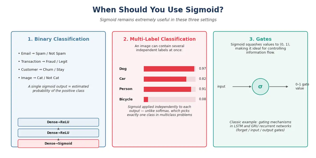
Sigmoid remains extremely useful.
1. Binary classification
Suppose the task is:
Email → Spam / Not Spam
Transaction → Fraud / Legitimate
Customer → Churn / Stay
Image → Cat / Not Cat
A single sigmoid output can represent the estimated probability of the positive class.
Typical architecture:
Dense → ReLU
        ↓
Dense → ReLU
        ↓
Dense → Sigmoid
2. Multi-label classification
Suppose an image can contain several independent labels:
Dog      = 0.97
Car      = 0.82
Person   = 0.91
Bicycle  = 0.08
A sigmoid can be applied independently to each output.
This differs from multiclass classification, where exactly one class may be selected and softmax is typically used.
3. Gates
Sigmoid-like gates are also useful when a model needs a value between 0 and 1 to control information flow.
A classic example is the gating mechanisms used in recurrent architectures such as LSTMs and GRUs.
When Should You Use ReLU?
ReLU is commonly used in hidden layers of:
- multilayer perceptrons
- convolutional neural networks
- image classification models
- computer vision systems
- many traditional deep neural network architectures
- feature-extraction networks
For a basic feed-forward network, a common starting point is:
Input
  ↓
Dense + ReLU
  ↓
Dense + ReLU
  ↓
Dense + ReLU
  ↓
Output activation appropriate to task
Google’s documentation recommends starting with ReLU when learning about activation functions.
Sigmoid vs ReLU: Decision Table
| Your requirement | Typical choice | Why |
|---|---|---|
| Hidden layer in basic deep network | ReLU | Efficient optimization |
| Binary classification output | Sigmoid | Maps logit to 0–1 |
| Multi-label classification | Sigmoid | Independent probabilities |
| Multiclass classification | Softmax | Produces normalized class distribution |
| Need negative hidden representations | Consider Tanh/GELU/etc. | ReLU clips negatives |
| Dead ReLU problem | Leaky ReLU/PReLU or other activation | Retains negative-side gradient |
| Traditional RNN gating | Sigmoid/Tanh | Useful bounded transformations |
| Modern Transformer-style architecture | Often GELU/SiLU-family | Architecture-specific design |
| Simple beginner network | ReLU hidden layers | Good starting point |
The key phrase is “typical choice,” not “mandatory choice.”
Architecture, initialization, normalization, optimizer, data distribution and objective function all affect the final decision.
Why ReLU Is Computationally Efficient
Sigmoid requires an exponential operation:
σ(x)=11+e−x\sigma(x)=\frac{1}{1+e^{-x}}
ReLU is simply:
max(0,x)max(0,x)
At a conceptual level, this makes ReLU much simpler to evaluate.
This difference becomes important when millions or billions of activations are calculated repeatedly during training and inference.
However, modern hardware libraries optimize activation functions heavily, so real-world training time is determined by the entire model and hardware stack, not by the mathematical operation alone.
Therefore, saying:
“ReLU is exactly X times faster than sigmoid”
without specifying hardware, tensor size, framework, precision, kernel implementation and workload would be misleading.
A Reproducible Benchmark Instead of a Made-Up Benchmark
A technically responsible article should not publish arbitrary speed numbers.
You can reproduce a simple benchmark with PyTorch:
import time
import torch

device = "cuda" if torch.cuda.is_available() else "cpu"

x = torch.randn(10_000_000, device=device)

# Warm-up
for _ in range(10):
    torch.relu(x)
    torch.sigmoid(x)

if device == "cuda":
    torch.cuda.synchronize()

start = time.perf_counter()

for _ in range(100):
    y = torch.relu(x)

if device == "cuda":
    torch.cuda.synchronize()

relu_time = time.perf_counter() - start

start = time.perf_counter()

for _ in range(100):
    y = torch.sigmoid(x)

if device == "cuda":
    torch.cuda.synchronize()

sigmoid_time = time.perf_counter() - start

print("Device:", device)
print("ReLU:", relu_time)
print("Sigmoid:", sigmoid_time)
This measures the activation operations on your actual environment rather than presenting a benchmark that may not generalize.
For serious performance analysis, use representative model workloads and profiling tools rather than isolated element-wise operations.
A Complete Binary Classification Example
Here is a simple TensorFlow/Keras implementation:
import tensorflow as tf

model = tf.keras.Sequential([
    tf.keras.layers.Input(shape=(20,)),
    tf.keras.layers.Dense(128, activation="relu"),
    tf.keras.layers.Dense(64, activation="relu"),
    tf.keras.layers.Dense(1, activation="sigmoid")
])

model.compile(
    optimizer="adam",
    loss="binary_crossentropy",
    metrics=["accuracy"]
)

model.summary()
The architecture is:
20 Input Features
       │
       ▼
Dense(128)
ReLU
       │
       ▼
Dense(64)
ReLU
       │
       ▼
Dense(1)
Sigmoid
       │
       ▼
Probability
The important architectural principle is:
Hidden layers learn representations; the output activation expresses the prediction format.
Sigmoid + Binary Cross-Entropy
For binary classification, sigmoid is commonly paired with binary cross-entropy.
The loss can be written as:
L=−[ylog(p)+(1−y)log(1−p)]L = -[y\log(p)+(1-y)\log(1-p)]
where:
- yy is the true label
- pp is the predicted probability
If:
y=1y=1
and:
p=0.95p=0.95
the loss is small.
If:
y=1y=1
but:
p=0.05p=0.05
the loss is large.
Important implementation detail
In many frameworks, it is preferable to provide raw logits to a numerically stable binary-cross-entropy-with-logits loss rather than manually applying sigmoid first.
For example, conceptually:
Dense(1)
   │
   ▼
Raw Logit
   │
   ▼
Binary Cross Entropy With Logits
rather than:
Dense(1)
   │
   ▼
Sigmoid
   │
   ▼
Binary Cross Entropy
Frameworks can implement the combined operation more stably, particularly for extreme logits.
This distinction matters when moving from educational examples to production ML systems.
The Difference Between Logits and Probabilities
This is one of the most commonly misunderstood parts of sigmoid-based classification.
Suppose the model produces:
z=3z=3
This is a logit, not a probability.
Applying sigmoid gives:
σ(3)≈0.953\sigma(3)\approx0.953
Now it can be interpreted as a probability-like output for a binary classifier.
Model output
    │
    │ z = 3.0
    ▼
 Sigmoid
    │
    │ p ≈ 0.953
    ▼
Probability
Understanding this distinction becomes particularly important when implementing loss functions, thresholding, calibration and deployment pipelines.
Architecture Matters More Than the Activation Function Alone
A common beginner mistake is to treat activation functions independently from the architecture.
In real deep learning systems, performance depends on interactions among:
- activation function
- initialization
- normalization
- optimizer
- learning rate
- batch size
- architecture depth
- architecture width
- loss function
- data distribution
- regularization
- hardware
- numerical precision
For example:
Activation
     │
     ├── Initialization
     │
     ├── Normalization
     │
     ├── Optimizer
     │
     ├── Learning Rate
     │
     └── Architecture
              │
              ▼
        Training Dynamics
Therefore, changing sigmoid to ReLU may improve optimization, but it does not automatically guarantee higher validation accuracy.
Edge Case: ReLU Can Produce Unbounded Positive Values
Unlike sigmoid:
0<σ(x)<10 < \sigma(x)<1
ReLU has no upper bound:
ReLU(x)→∞ReLU(x)\rightarrow\infty
as x→∞x\rightarrow\infty.
This can be useful because positive activations are not compressed.
But it also means activation magnitude can become large under some circumstances.
This is one reason why initialization, normalization and optimization settings matter.
Edge Case: ReLU Is Not Differentiable at Zero
Strictly speaking, ReLU has a kink at:
x=0x=0
The left derivative is:
00
while the right derivative is:
11
So the classical derivative does not exist exactly at zero.
Deep learning frameworks nevertheless define a practical gradient convention at that point.
This illustrates an important distinction between the mathematical idealization of an activation function and its implementation inside automatic differentiation systems.
Edge Case: Numerical Stability With Sigmoid
Directly evaluating:
e−xe^{-x}
can become numerically problematic for very large positive or negative values.
Production implementations therefore use numerically stable kernels.
This is another reason not to implement low-level activation functions casually when a mature framework already provides optimized implementations.
TensorFlow’s sigmoid implementation is provided as part of its activation API.
ReLU in Convolutional Neural Networks
A simplified CNN architecture might look like:
Image
 │
 ▼
Conv2D
 │
 ▼
ReLU
 │
 ▼
Pooling
 │
 ▼
Conv2D
 │
 ▼
ReLU
 │
 ▼
Pooling
 │
 ▼
Dense
 │
 ▼
Output
For example, a computer-vision model could use ReLU after convolutional layers to introduce nonlinearity into learned feature maps.
The network may progressively learn representations such as:
Pixels
  ↓
Edges
  ↓
Textures
  ↓
Shapes
  ↓
Object Parts
  ↓
Objects
The activation function is only one component of this hierarchy, but its gradient behavior affects whether the network can efficiently learn these transformations.
Why ReLU Enabled Deeper Networks
The historical importance of rectifier activations is larger than simply replacing sigmoid with a different curve.
Deep networks are difficult to optimize because gradients must propagate through many transformations.
Rectifier-based approaches helped make deeper networks practical.
The 2015 PReLU research by He, Zhang, Ren and Sun investigated rectifier nonlinearities and proposed a parameterized rectifier together with an initialization method designed for very deep rectifier networks.
This work is part of the broader development that led to highly successful deep convolutional architectures.
Sigmoid vs ReLU for Different ML Problems
| Problem | Hidden Layers | Output Layer |
|---|---|---|
| Binary classification | ReLU or suitable modern activation | Sigmoid |
| Multi-label classification | ReLU or suitable modern activation | Sigmoid per label |
| Multiclass classification | ReLU or suitable modern activation | Softmax |
| Regression | ReLU or suitable modern activation | Linear |
| Image classification | Often ReLU-family or architecture-specific activation | Task-dependent |
| Sequence modeling | Architecture-dependent | Task-dependent |
| Gated recurrent networks | Architecture-specific | Often sigmoid/tanh internally |
This table is intentionally architecture-aware.
There is no universal rule that every neural network should use ReLU everywhere.
Common Myths About Sigmoid vs ReLU
Myth 1: Sigmoid is obsolete
False.
Sigmoid is still highly useful when a bounded 0–1 output is appropriate.
It remains common for binary classification outputs and gating mechanisms.
Myth 2: ReLU always gives better accuracy
False.
ReLU often improves optimization characteristics, but final model quality depends on architecture, data, optimization and task.
Better gradient flow does not mathematically guarantee better generalization.
Myth 3: ReLU completely eliminates vanishing gradients
False.
ReLU reduces one important source of vanishing gradients on its positive branch, but neural networks can still experience vanishing or exploding gradients for other reasons.
Myth 4: ReLU has no gradient problem
False.
The negative branch has zero gradient, which can produce dead neurons.
Myth 5: Sigmoid should never appear inside a neural network
False.
Sigmoid is particularly useful when a model needs a bounded gate or binary probability output.
Practical Decision Framework
When selecting an activation function, ask these questions in order.
Question 1: Is this a hidden layer or output layer?
This is often the most important distinction.
Question 2: What does the output represent?
Probability?
Continuous value?
Class distribution?
Feature representation?
Gate?
Question 3: Can saturation damage gradient flow?
If yes, consider whether sigmoid or tanh is appropriate.
Question 4: Can zero gradients on negative inputs become a problem?
If yes, consider Leaky ReLU, PReLU or another activation.
Question 5: Does the architecture have a standard activation?
Modern architectures frequently specify their activation as part of the architecture itself.
Question 6: Have you validated the choice experimentally?
For production systems, activation selection should ultimately be evaluated using the actual dataset, training procedure and validation protocol.
A Practical Activation-Function Workflow
                    Start
                      │
                      ▼
             What is the layer?
               /            \
          Hidden             Output
            │                  │
            ▼                  ▼
   Start with architecture   What is the
   appropriate activation     target?
            │              /     |      \
            │        Binary   Multi   Regression
            │          │       class      │
            │          ▼         ▼         ▼
            │       Sigmoid   Softmax    Linear
            │
            ▼
      Monitor training
            │
            ▼
   Vanishing gradients?
        /          \
      Yes           No
       │             │
       ▼             ▼
 Consider ReLU/    Monitor
 alternatives     validation
       │
       ▼
 Dead ReLU units?
       │
      Yes
       │
       ▼
 Consider Leaky
 ReLU / PReLU /
 other activation
Sigmoid vs ReLU: The Short Technical Answer
If you need a concise technical rule:
Use ReLU or an architecture-appropriate ReLU-family/modern activation as a starting point for many hidden layers because its positive-side derivative avoids the strong saturation associated with sigmoid.
Use sigmoid when the mathematical meaning of a bounded 0–1 output is useful, particularly for binary or multi-label outputs and gating mechanisms.
That distinction is much more useful than simply saying:
“ReLU is better than sigmoid.”
Frequently Asked Questions
Is ReLU better than sigmoid?
For many hidden layers in deep neural networks, ReLU is a more practical default because its positive branch has a gradient of 1 and is less susceptible to sigmoid-style saturation.
However, sigmoid remains the appropriate choice for several tasks, particularly binary-output layers.
Why does sigmoid cause vanishing gradients?
Sigmoid saturates toward 0 and 1. Its derivative becomes very small in those regions. During backpropagation, repeatedly multiplying small derivatives across layers can make gradients extremely small.
Why is ReLU faster than sigmoid?
ReLU is mathematically simple:
max(0,x)max(0,x)
Sigmoid requires an exponential calculation.
However, actual performance depends on optimized framework kernels, hardware, tensor sizes and the complete neural-network workload.
Can ReLU and sigmoid be used in the same model?
Yes.
A common binary-classification architecture can use:
Hidden Layer → ReLU
Hidden Layer → ReLU
Output Layer → Sigmoid
The two functions serve different purposes.
Why does ReLU produce zero for negative inputs?
The definition is:
ReLU(x)=max(0,x)ReLU(x)=max(0,x)
Therefore every negative input becomes zero.
This creates sparse activations, which can be useful, but it can also contribute to dead neurons.
What is a dead ReLU?
A dead ReLU is a neuron that consistently receives negative pre-activation values and therefore outputs zero with a zero gradient on that branch.
If this persists, the neuron may stop learning.
What can replace ReLU?
Common alternatives include:
- Leaky ReLU
- PReLU
- ELU
- GELU
- SiLU/Swish
- Mish
- SELU
The correct choice depends on the architecture and training objective.
TensorFlow currently provides many of these activation functions through its Keras activation API.
Should beginners learn sigmoid before ReLU?
Yes.
Sigmoid is conceptually important because it makes the relationship between activation functions, probability outputs, derivatives and vanishing gradients easier to understand.
ReLU then provides a natural introduction to modern deep-network optimization.
Final Verdict: Sigmoid vs ReLU
The sigmoid vs ReLU debate is not really about choosing one universal winner.
The functions solve different problems.
Sigmoid is bounded, smooth and naturally suited to representing binary probabilities and gates. Its weakness is saturation, which can cause very small gradients and make it difficult to optimize deep hidden layers.
ReLU is simple, computationally efficient and has a constant positive-side derivative. This makes it an effective default for many hidden layers. Its main weakness is the possibility of dead neurons caused by its zero-gradient negative branch.
A practical deep-learning architecture therefore often looks like:
                Input
                  │
                  ▼
             Dense / Conv
                  │
                ReLU
                  │
                  ▼
             Dense / Conv
                  │
                ReLU
                  │
                  ▼
              Output
                  │
        ┌─────────┴─────────┐
        │                   │
     Binary              Multiclass
        │                   │
     Sigmoid             Softmax
The deeper lesson is that activation functions should be selected according to the role of the layer, the optimization behavior of the architecture, and the mathematical meaning of the output.
That is why modern deep learning does not simply ask, “Sigmoid or ReLU?”
It asks:
“What transformation does this layer need, and which activation gives the model the right representation and gradient behavior for that job?”

AiVoogle – AI Tutorials & AI Tools
AiVoogle is an AI-focused platform sharing practical AI tutorials, AI tools, guides, reviews, and the latest trends in artificial intelligence. Our goal is to make AI simple, useful, and accessible for everyone—from beginners and creators to marketers, developers, and businesses.
The AiVoogle team researches and covers the latest AI tools and technologies to help readers discover the right tools and learn how to use AI effectively.
Focus: AI Tutorials | AI Tools | AI Guides | AI News | AI Reviews